
This comes from the file content/analysis.Rmd.
Author: Liangxi Dou, Jialin Guo, Yutong Du and Jiaqi Yin.
Hypothesis:
- The well-being of customers often stand at the core of a banking service. It might not be a huge issue when a few customers leave the bank’s services. But as the number of churning customers accumulate, the effects gradually alleviate. Nowadays, more and more banks start to become frustrated to see their customers drop out from their services and turn to another bank seemingly out of no reason.
- There is always a reason behind a churn. In this project, we look at datasets collected by a company manager that records several important personal information in regards to their registered customers. Some of them still stay with the bank, some of them have already churned.
- We aim to take a deep dive into these different factors and find out what exactly affects customer churning or what’s the determining factor for attried customers.
- Initially, we intend to look at eight different factors that could potentially affect churning. They are: customer age,gender, education level, incomes, total transaction amount, total transaction counts, revolving balance on card and card utilization rate.
- Gender
- education level
- Income level
- Total Transaction Amount
- Total Transaction Counts
- Revolving Balance on card
- Card Utilization rate
Gender
 Analysis:
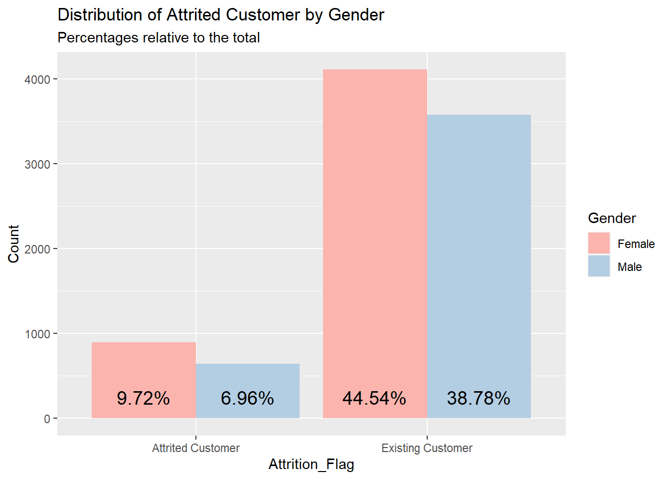
- In first dataset, we notice that the majority of customers(83.93%) are still existing customers, and as 43.72%>40.21% and 9.18%>6.88% hence, the number of female customers is greater than males. From here, we may say that female customers tend to churn more often, and gender may potentially play a role in customer churning
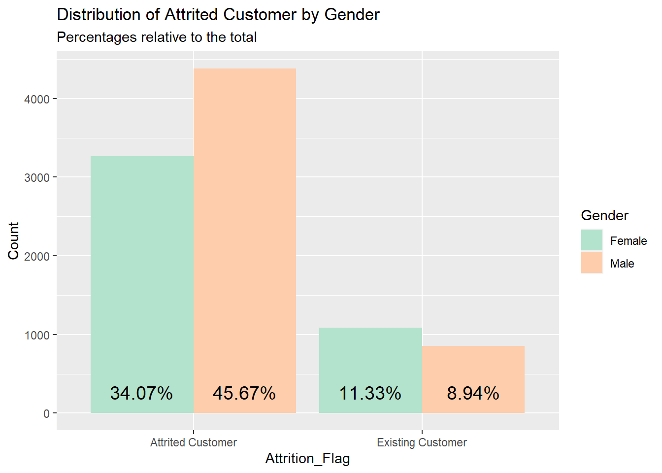
- However, in our second dataset, we see a completely different situation. We find out that around 80%(79.63% to be exact) of customers have already been attrited customers, and it is not the case that female card holders usually tend to churn more often than males(as 34%<45%). Instead, there are more male customers that churn.
- Although there might be potential bias around data collection methods, yet we are still able to draw the conclusion that AGE is not the determining factor of customer churning and being male or female customer does not really make a difference.
Education_Level
 Analysis:
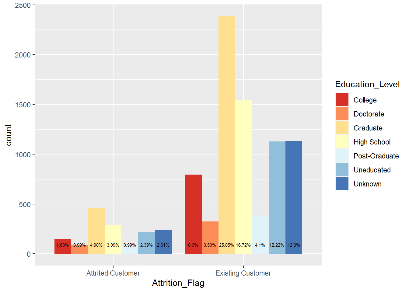
- At first glance, we might say that it seems people at graduate level them to have the most customer churning rate and the second one is high school, then follows with undergraduate and unknown groups.
- But this is hardly the case. To better understand the relationship between customer churning and education level, we need to look at the exact percentage or proportion of Attrition rate(num of attrited/existed). After some calculations, we find out that range from college to unknown customers, attrition rate tends to be similar. For college students, the attrition rate is 17.9%; for doctoral students is 26.7%; for graduate student is 18.44%; high school student is 17.91%. The percentage ranges from 15%-20% and follows no clear trend. Although graduate students have the most population of card holders, they do not have the most attrition rate. Hence, we conclude that Education level is not closely related to whether customers will churn or not. It is not the determining factor.
Income_category
## Warning: ³Ì¼°ü'fmsb'ÊÇÓÃR°æ±¾4.0.3 À´½¨ÔìµÄ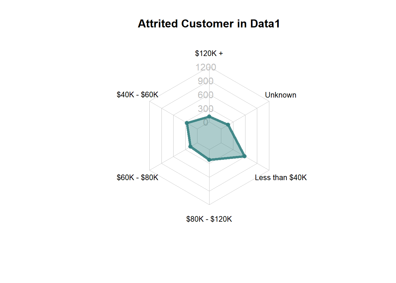
 Analysis:
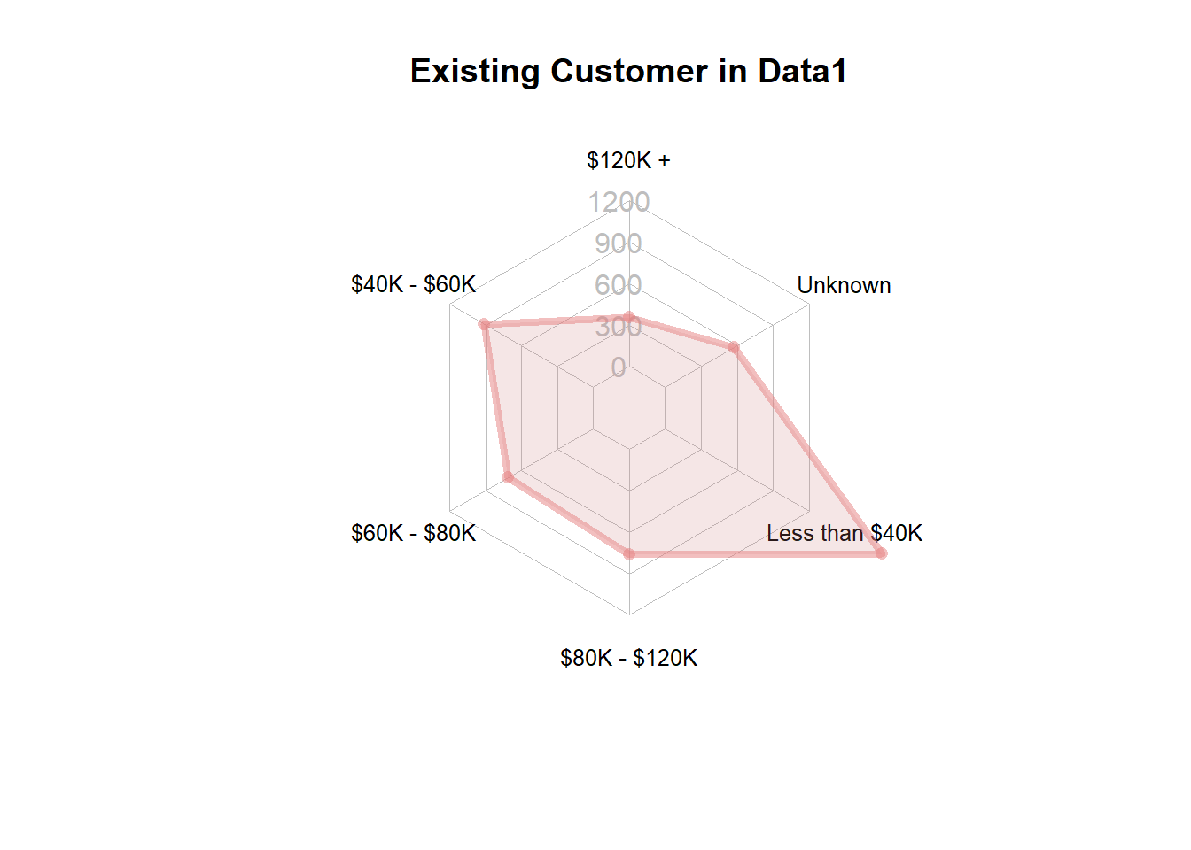
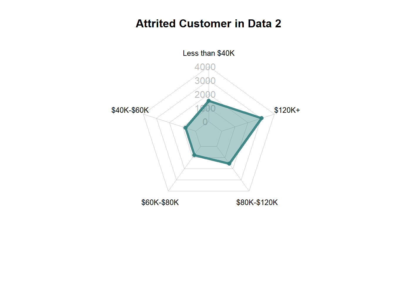
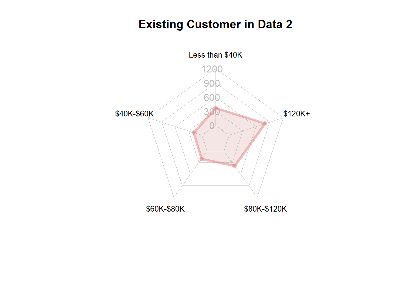
- As we see in first dataset’s radar chart, at various income level, the number of existing and attrited customers seem have similar spread. Most existing customers fall into the group of less than $40k, and the same as attrited customers. For unknown category, it contains the least number of existing customers which is also the same situation for attrited customers. In the second graph, we also notice this same trend whereas the population of existing customers increases, the number of attrited customers in that income category also increases.
- This is the same case as previously what we see in Education_Level. Hence, we conclude that clients income categories really affect whether or not they will churn. In short, income category is also not the determining factor of churning.
Total Transactions Counts
Analysis:
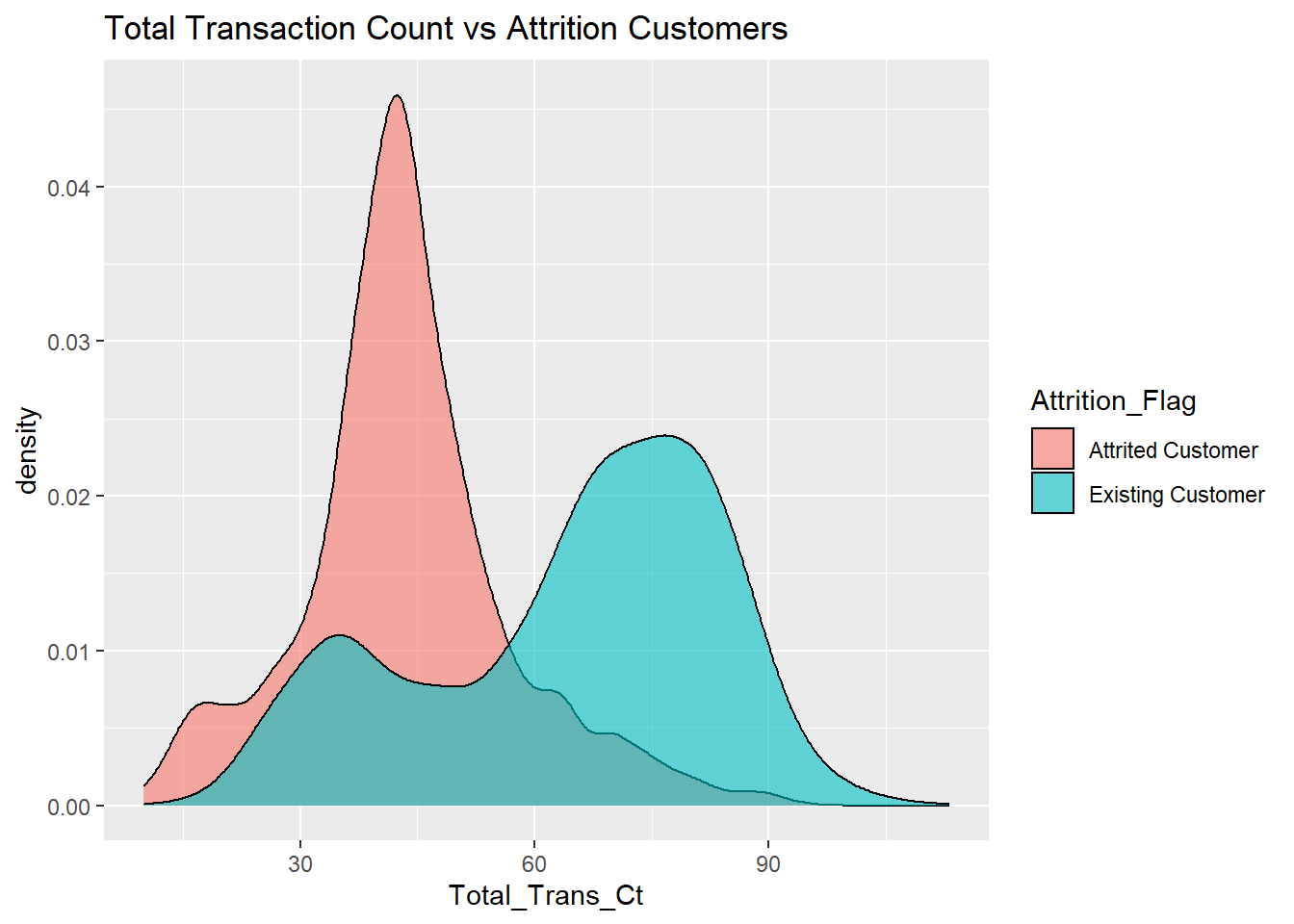
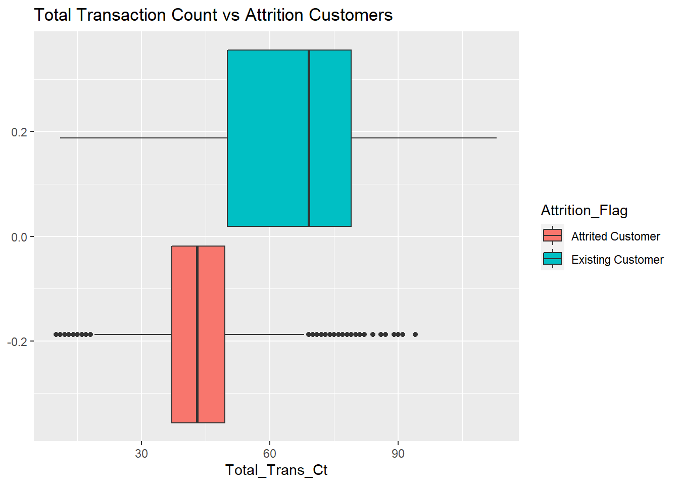
- Now we are looking at the comparison between attired and exited customers on total transaction counts. The counts represent the frequency of how many times a card holder uses the card each month. From the First graph, we notice that the density of attired customers’ total transaction count meets its max at around 50times, while the max point for existing customers is at around 75times per month. They tend to be bell-shaped. Most attired customers only use them cards around 50 times per month. Hence, it’s clear to interpret that attired customers tend to use their card much less times compared with active customers.
- From the box plot above, we could see that 50% of customers who left credit card services had a number of transactions in the last 12 months less than or equal to 43. Most importantly, from interpreting the upper quartile, we can see that 75% of customers who left credit card services had a number of transactions in the last 12 months less than or equal to 51. While the lower quartile of existing customers have a transaction count that is higher than that. The median of the people who remained with the card services is 71 transactions and the third quartile of people who remained with card services is 82 transactions. These cope with our previous analysis on the distribution between Total Transaction Count vs Attrition Customer and further prove that higher frequency of transaction usually means higher chance of staying with the credit card service.
- Combining our findings in both graphs, we can conclude that the smaller the total transactions counts for a customer, then more likely this customer will become attrited. Hence, total transaction count is the determining factor for customer churning.
Total Transaction Amount
 Analysis:
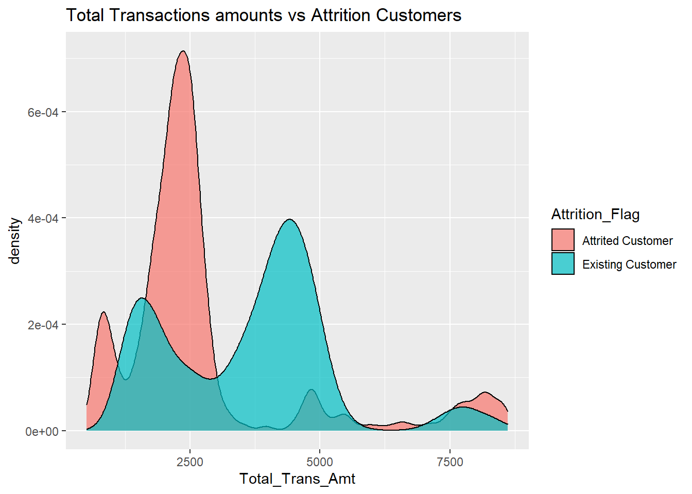
- In the first plot, we notice that distribution of attrited customer tend to be skewed left. The amount of money that attired customer transferred seem to have a much narrower range(around 0-3000) and max at around 2500. Although we can see some graph around 5000-7500, but majority of churned customer only transfer small amount of money. For existing customers, their total transaction amounts have a much wider range. They range from 0-7500 and have two max points, at around 2000 and around 4375. But when looking at density, we notice attrited customers have a much higher density at its max point compared with existing customers. It reveals that most attrited customers only transfer a very small portion of money yearly based, while active customers transfer a wide range of amount. Some of them transfer more, small less.
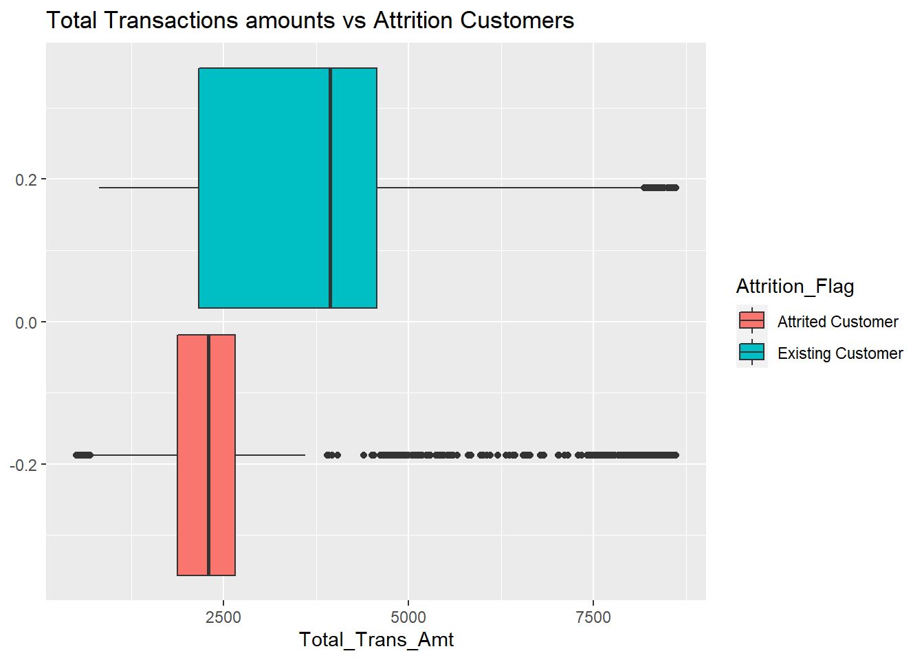
- In the box-plot, we have a much clearer picture towards the comparison between the two. As we see, the box-plot of attrited customers is much thinner compared with existing customers. This shows that most churned customers only transfer a small portion of money with their card yearly. Moreover, we see the lower percentile of total transition amounts for existing customers is almost equal to the median of total transition amounts for attrited customers. The true median of existing customers lie above 3750. Hence, we are able to conclude that Total Transaction Amount is the determining factor of churning customers.
Total Revolving Balance
 Analysis:
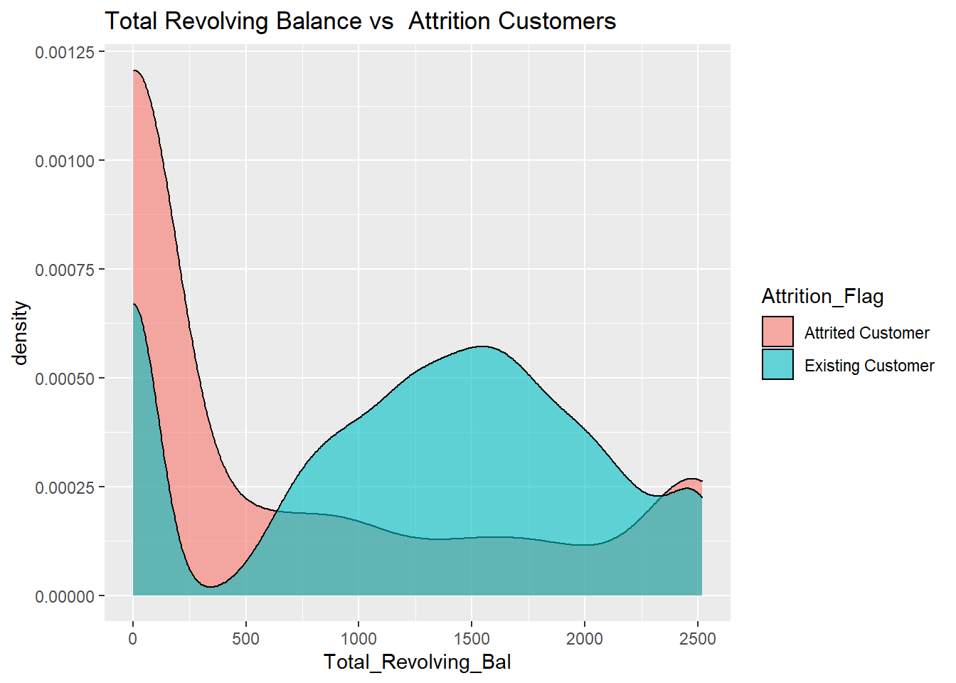
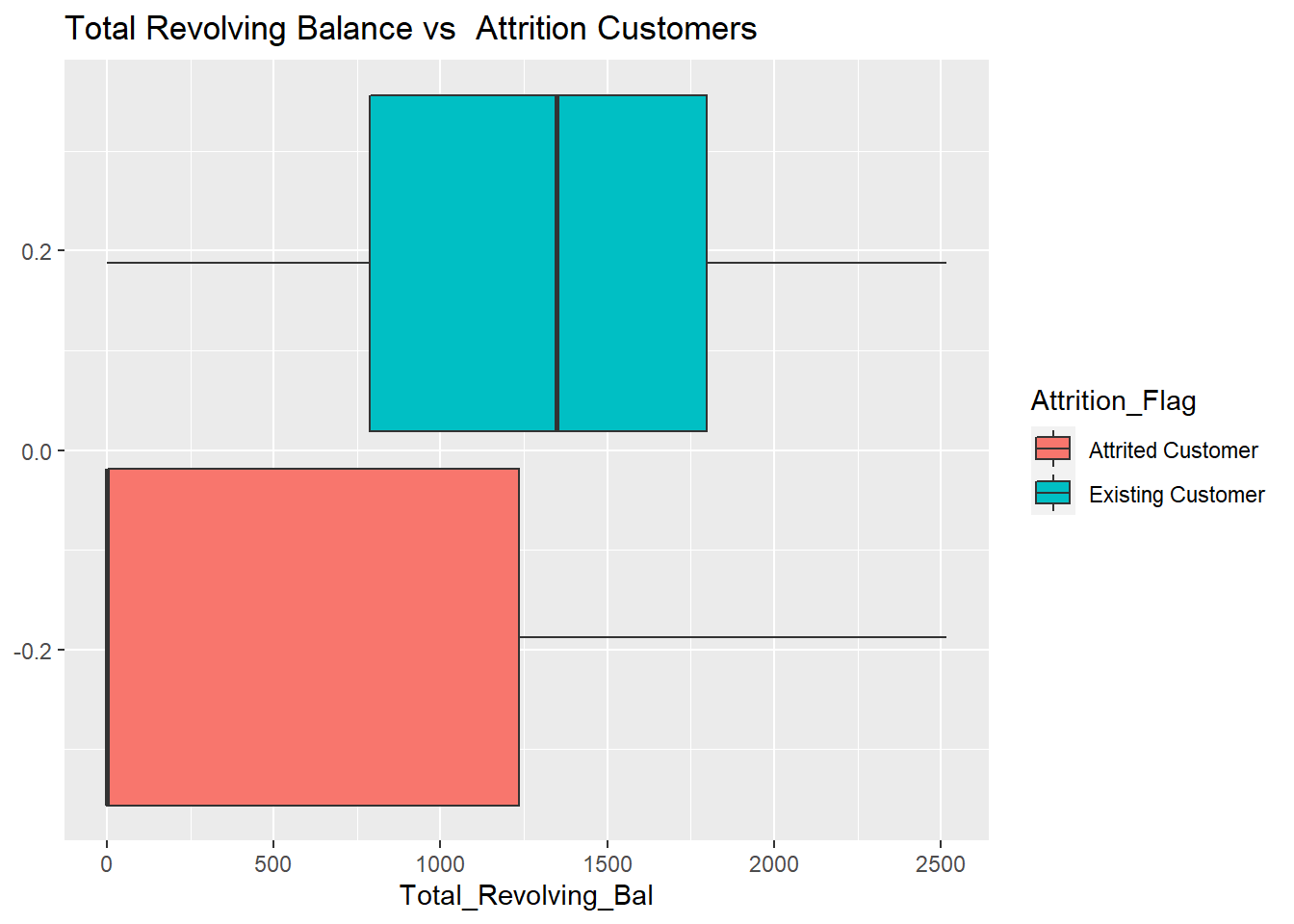
- In first plot, we clearly see that the graph of revolving balance in cards for attrited holders tend to be extremely skewed left, and for most customers their balance tend to be zero or somewhere around zero. But for existing customers, their balance ranges from 0-2500, and density meets its max point at around 1500.
- In box-plot, the difference between attrited and existing customers seem to be more apparent. In the red colored plot, the lower percentile lies at 0 and upper percentile at around 1250. For existing customers, it has a median of above 1300 and lower percentile at around 750, upper at above 1570. There is a clear difference between churned and active customers. In this way, we can safely draw the conclusion that the attrited customer has much lower or even no balance remaining in their account and existing customer has higher balance and a wider range of balance. Total Revolving Balance is the determining factor to decide whether a client will churn or not.
Average Card Ultralization Rate
 Analysis:
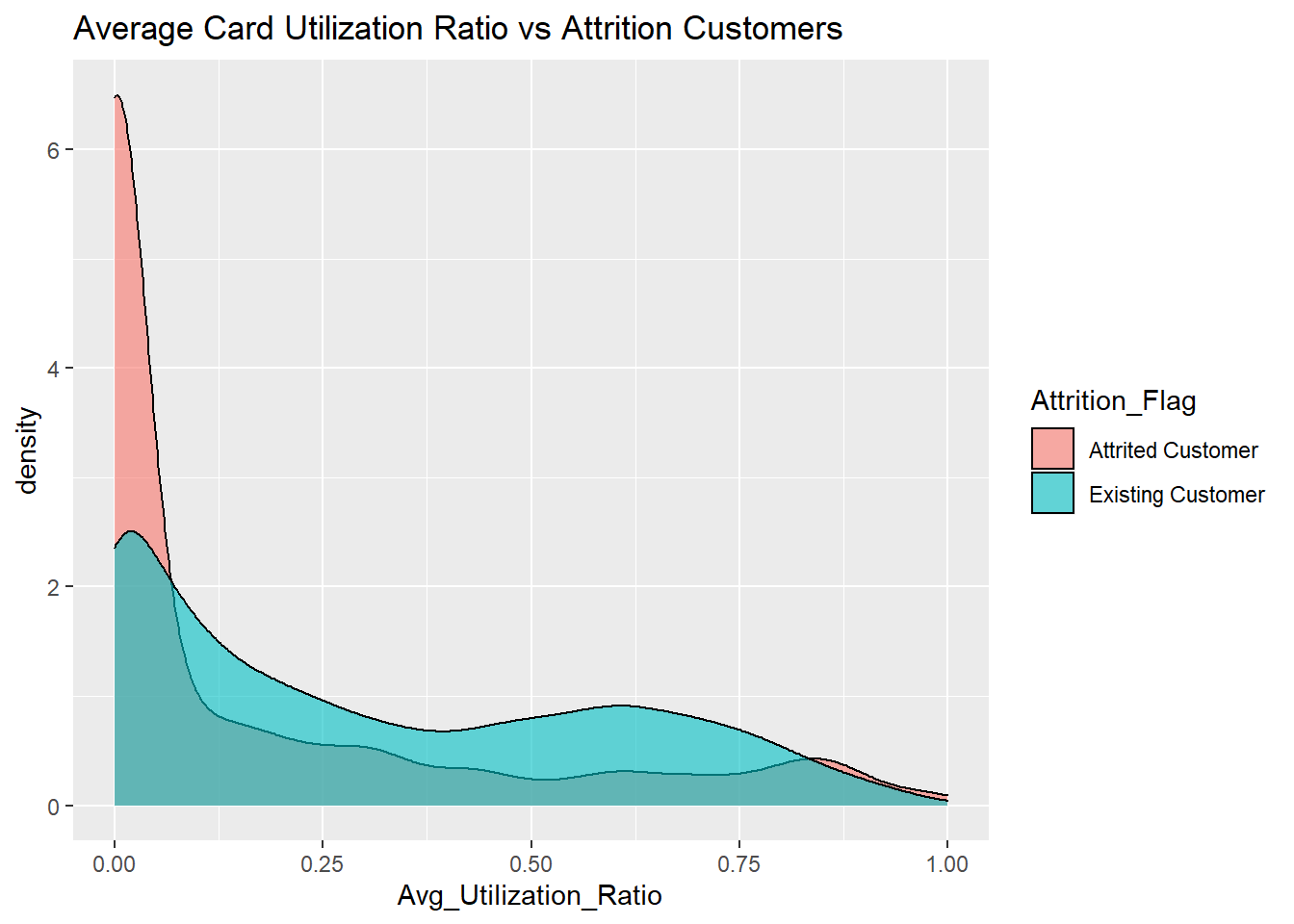
- Similar conditions with total revolving balance. We notice a clear trend that the ultralization rate for attrited customers is low and mostly below 25%, while for existing customers their utilization rate spans the entire x-axis and ranges from 0% to 100%. It seems that when a customer starts to use their card less and less times, there is a higher chance for him or her to become churned.
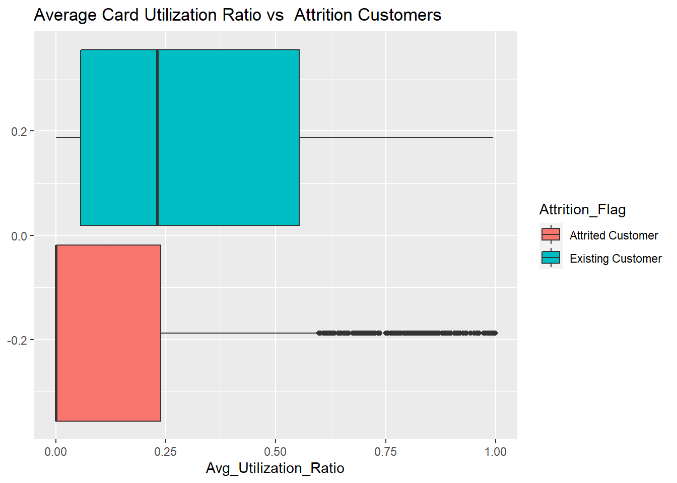
- To get a closer look at this phenomenon, in box-plot, the median of existing customers lie at somewhere around 25%, while for attrited customers it is 0%. The 75th percentile for churned customers is almost the same as existing customers. Not to mention the IQR of attrited customers is also much smaller than existing. Therefore, as both graphs prove the point that customers with low utilization rate(below 25%) tend to become churned. An average utilization rate is the determining factor in customer churning.
Model Perdiction
- Our goal for the Model section is to predict which groups of factors will impact a customer’s decision of leaving the bank or not(Attrition_Flag). According to the EDA section, we analyzed factors that we believe are influential to the customer decision and displayed four impactive factors. In order to get a more accurate model to discuss the factors impact on a customer’s decision of leaving a bank or not, more variables that may correlate with the customer’s decision are included in this Model section.
Correlation Map
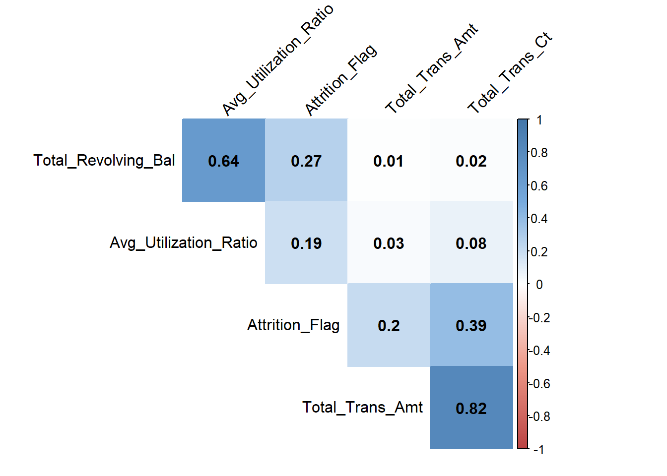 The correlation matrix shows the correlation between the four variables displayed in EDA. According to the matrix, Total_Trans_Ct(Total Transaction Count) and Total_Trans_Amt(Total Transaction Amount) are highly correlated. Though factor Total_Revolving Bal and Avg_Utilization_Ratio is also related, Avg_Utilization_Ratio will be removed from the model selection as it has less significance.
Model1
##
## Call:
## glm(formula = Attrition_Flag ~ Total_Trans_Ct + Total_Trans_Amt +
##     Total_Revolving_Bal + Avg_Utilization_Ratio, family = binomial)
##
## Deviance Residuals:
##     Min       1Q   Median       3Q      Max
## -3.3681   0.1150   0.2500   0.4799   2.4199
##
## Coefficients:
##                         Estimate Std. Error z value Pr(>|z|)
## (Intercept)           -3.602e+00  1.241e-01 -29.029   <2e-16 ***
## Total_Trans_Ct         1.283e-01  3.840e-03  33.400   <2e-16 ***
## Total_Trans_Amt       -8.361e-04  3.836e-05 -21.797   <2e-16 ***
## Total_Revolving_Bal    1.176e-03  6.076e-05  19.351   <2e-16 ***
## Avg_Utilization_Ratio -4.224e-01  1.833e-01  -2.305   0.0212 *
## ---
## Signif. codes:  0 '***' 0.001 '**' 0.01 '*' 0.05 '.' 0.1 ' ' 1
##
## (Dispersion parameter for binomial family taken to be 1)
##
##     Null deviance: 8318.8  on 9227  degrees of freedom
## Residual deviance: 5601.5  on 9223  degrees of freedom
## AIC: 5611.5
##
## Number of Fisher Scoring iterations: 6
## Start: AIC=5611.53
## Attrition_Flag ~ Total_Trans_Ct + Total_Trans_Amt + Total_Revolving_Bal +
## Avg_Utilization_Ratio
##
## Df Deviance AIC
## <none> 5601.5 5611.5
## - Avg_Utilization_Ratio 1 5606.8 5614.8
## - Total_Revolving_Bal 1 6052.1 6060.1
## - Total_Trans_Amt 1 6113.5 6121.5
## - Total_Trans_Ct 1 7203.6 7211.6## [1] 0.8672518According to our EDA analysis, we first choose four different variables to conduct our logistic regression. Since our dependent variable is a categorical variable, we choose to plot a logistic curve. Then, based on these four variables, we create the model and by using threshold = 0.5, we are able to measure our accuracy to be 86.7%, which is pretty high and can be representative of our entire data. Every variable in this model is statistically significant for a = 0.05.
Model2
##
## Call:
## glm(formula = Attrition_Flag ~ Total_Trans_Ct + Total_Trans_Amt +
##     Total_Revolving_Bal + Avg_Utilization_Ratio + Total_Trans_Amt *
##     Total_Trans_Ct, family = binomial, data = Bank_new)
##
## Deviance Residuals:
##     Min       1Q   Median       3Q      Max
## -3.4440   0.0620   0.2061   0.4788   2.6393
##
## Coefficients:
##                                  Estimate Std. Error z value Pr(>|z|)
## (Intercept)                    -4.494e-01  2.328e-01  -1.931   0.0535 .
## Total_Trans_Ct                  8.177e-02  5.068e-03  16.133   <2e-16 ***
## Total_Trans_Amt                -2.612e-03  1.263e-04 -20.684   <2e-16 ***
## Total_Revolving_Bal             1.090e-03  6.111e-05  17.838   <2e-16 ***
## Avg_Utilization_Ratio          -2.190e-01  1.854e-01  -1.181   0.2377
## Total_Trans_Ct:Total_Trans_Amt  2.609e-05  1.779e-06  14.663   <2e-16 ***
## ---
## Signif. codes:  0 '***' 0.001 '**' 0.01 '*' 0.05 '.' 0.1 ' ' 1
##
## (Dispersion parameter for binomial family taken to be 1)
##
##     Null deviance: 8318.8  on 9227  degrees of freedom
## Residual deviance: 5330.2  on 9222  degrees of freedom
## AIC: 5342.2
##
## Number of Fisher Scoring iterations: 7
## [1] 0.8794972Through a correlation map, we could find out that the Total_Trans_Amt and Total_Trans_Ct has strong correlation. Hence, we add an interactive term of Total Transaction Amount and Total Transaction Count. The accuracy of this model is 87.95%, which is higher than model 1. However, the p-value of Avg_Utilization_Ratio is greater than 0.05,so this variable is not statistically significant at α = 0.05.
Model3
##
## Call:
## glm(formula = Attrition_Flag ~ Total_Trans_Ct + Total_Trans_Amt +
##     Total_Revolving_Bal + Total_Trans_Amt * Total_Trans_Ct, family = binomial,
##     data = Bank_new)
##
## Deviance Residuals:
##     Min       1Q   Median       3Q      Max
## -3.4354   0.0617   0.2066   0.4786   2.6071
##
## Coefficients:
##                                  Estimate Std. Error z value Pr(>|z|)
## (Intercept)                    -4.329e-01  2.322e-01  -1.864   0.0623 .
## Total_Trans_Ct                  8.130e-02  5.045e-03  16.114   <2e-16 ***
## Total_Trans_Amt                -2.618e-03  1.263e-04 -20.720   <2e-16 ***
## Total_Revolving_Bal             1.040e-03  4.364e-05  23.835   <2e-16 ***
## Total_Trans_Ct:Total_Trans_Amt  2.620e-05  1.778e-06  14.738   <2e-16 ***
## ---
## Signif. codes:  0 '***' 0.001 '**' 0.01 '*' 0.05 '.' 0.1 ' ' 1
##
## (Dispersion parameter for binomial family taken to be 1)
##
##     Null deviance: 8318.8  on 9227  degrees of freedom
## Residual deviance: 5331.6  on 9223  degrees of freedom
## AIC: 5341.6
##
## Number of Fisher Scoring iterations: 7
## [1] 0.8792805We take out Avg_Utilization_Ratio in model 3 and the final accuracy is 87.93, which is almost the same with the accuracy in model2. However, every variable in this model is statistically significant at α= 0.05.
Model4
##
## Call:
## glm(formula = Attrition_Flag ~ Total_Trans_Ct + Total_Trans_Amt +
##     Total_Revolving_Bal + Avg_Utilization_Ratio + Total_Trans_Amt *
##     Total_Trans_Ct + Gender + Months_on_book + Marital_Status,
##     family = binomial, data = Bank_new)
##
## Deviance Residuals:
##     Min       1Q   Median       3Q      Max
## -3.5764   0.0607   0.2007   0.4655   2.7726
##
## Coefficients:
##                                  Estimate Std. Error z value Pr(>|z|)
## (Intercept)                    -1.265e+00  3.316e-01  -3.813 0.000137 ***
## Total_Trans_Ct                  9.161e-02  5.254e-03  17.435  < 2e-16 ***
## Total_Trans_Amt                -2.530e-03  1.268e-04 -19.955  < 2e-16 ***
## Total_Revolving_Bal             9.734e-04  6.263e-05  15.542  < 2e-16 ***
## Avg_Utilization_Ratio           1.923e-01  1.961e-01   0.981 0.326662
## GenderM                         6.271e-01  7.507e-02   8.354  < 2e-16 ***
## Months_on_book                 -1.096e-03  4.271e-03  -0.257 0.797419
## Marital_StatusMarried           3.668e-01  1.438e-01   2.551 0.010751 *
## Marital_StatusSingle           -1.590e-01  1.451e-01  -1.095 0.273310
## Marital_StatusUnknown          -5.828e-02  1.849e-01  -0.315 0.752664
## Total_Trans_Ct:Total_Trans_Amt  2.454e-05  1.790e-06  13.708  < 2e-16 ***
## ---
## Signif. codes:  0 '***' 0.001 '**' 0.01 '*' 0.05 '.' 0.1 ' ' 1
##
## (Dispersion parameter for binomial family taken to be 1)
##
##     Null deviance: 8318.8  on 9227  degrees of freedom
## Residual deviance: 5211.9  on 9217  degrees of freedom
## AIC: 5233.9
##
## Number of Fisher Scoring iterations: 7
## [1] 0.8810143To get a more accurate model to predict customers’ decisions, we also add some other variables that may be correlated with customers’ decisions, like gender, months_on_book(Customer’s period of relationship with bank), and marital_status. However, after we summarized model4, we found that most of the new variables don’t have significance at α=0.05. Even though the accuracy value is higher than model3, we believe it is because more variables are considered.
Accuracy of Model1
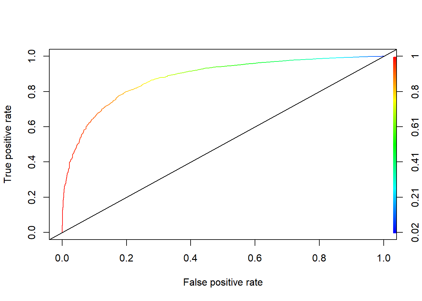
## [1] 0.8770522Accuracy of Model2

## [1] 0.8890957Accuracy of Model3
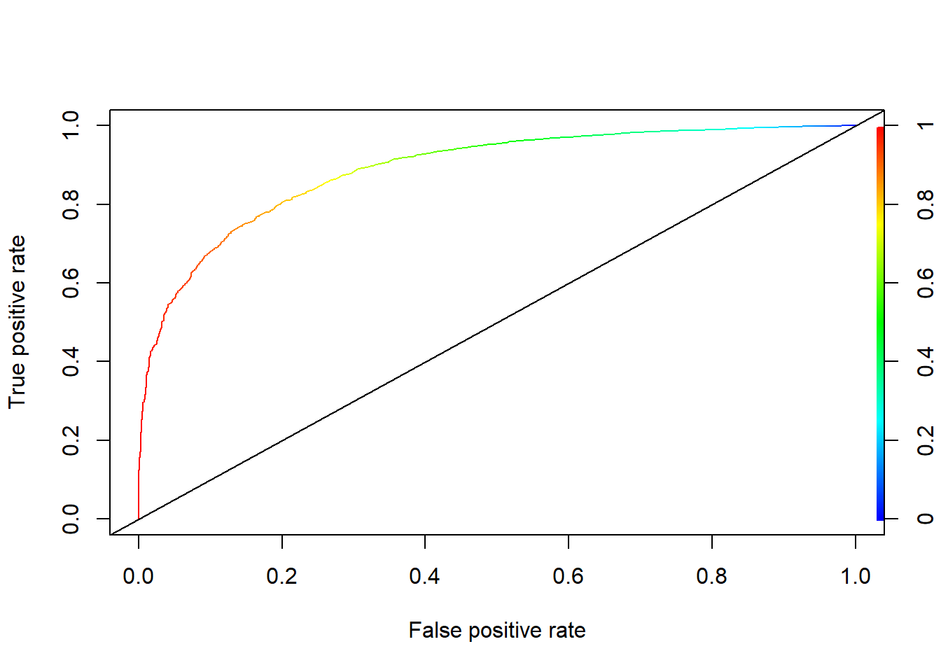
## [1] 0.8892446Accuracy of Model4

## [1] 0.8892446The above four pictures are ROC graphs of four models. An ROC curve (receiver operating characteristic curve) is a graph showing the performance of a classification model at all classification thresholds. When the ROC curve is closer to the point(0,1), the model has better effect. We use the area under the curve to measure the effectiveness of the model and the way to measure this area is AUC. When AUC is bigger, the model is better effective. Model 3 and Model 4 have the highest AUC value and even almost the same value.
Conclusion:
- In conclusion, after comparing four different models, we choose the third model. We believe that two factors potentially may influence the fluctuation of accuracy level. First, the number of variables present in a model. As more variables exist, it may cause the level of accuracy to increase. Such increase is not desired, hence we wish to limit the amount of variables present. Under such conditions, we are done to Model 1 and 3, which contains four variables. Second, we look at the accuracy level. At glance, we notice that Model 3 and 4 have a higher accuracy level. But in model 4, the variable it uses tends to be less significant compared with model 3. Also, according to the correlation map, we find out there’s a high correlation between total transaction amounts and transaction counts. Hence, we think model 3 is the best fit model we have that better predict customer churning.
- And due to limitations of variable and potential bias exist in dataset, since only 16.07% of overall customers churned, this model may not be as accurate as it sounds. Further studies and analysis are still needed for a more precise model.