# Based on the unique character of our dataset, we use both linear regression and logistic regression for our models. We try to predict whether a customer will end their use of the credit card company or continue with the company based on different variables including Marital_Status, Education level and Income level.

library(tidyverse)
## ── Attaching packages ─────────────────────────────────────── tidyverse 1.3.0 ──## ✓ ggplot2 3.3.3 ✓ purrr 0.3.4
## ✓ tibble 3.0.5 ✓ dplyr 1.0.3
## ✓ tidyr 1.1.2 ✓ stringr 1.4.0
## ✓ readr 1.4.0 ✓ forcats 0.5.0## ── Conflicts ────────────────────────────────────────── tidyverse_conflicts() ──
## x dplyr::filter() masks stats::filter()
## x dplyr::lag() masks stats::lag()library(modelr)
BankChurners <- read_csv("BankChurners.csv")##
## ── Column specification ────────────────────────────────────────────────────────
## cols(
## .default = col_double(),
## Attrition_Flag = col_character(),
## Gender = col_character(),
## Education_Level = col_character(),
## Marital_Status = col_character(),
## Income_Category = col_character(),
## Card_Category = col_character()
## )
## ℹ Use `spec()` for the full column specifications.Attrition_Flag=as.factor(BankChurners$Attrition_Flag)
Attrition_Flag=as.numeric(Attrition_Flag)
Gender=as.factor(BankChurners$Gender)
Gender=as.numeric(Gender)
Marital_Status=as.factor(BankChurners$Marital_Status)
Marital_Status=as.numeric(Marital_Status)
Education_Level=as.factor(BankChurners$Education_Level)
Education_Level=as.numeric(Education_Level)
Income_Category=as.factor(BankChurners$Income_Category)
Income_Category=as.numeric(Income_Category)
Card_Category=as.factor(BankChurners$Card_Category)
Card_Category=as.numeric(Card_Category)
Customer_Age=as.factor(BankChurners$Customer_Age)
Customer_Age=as.numeric(Customer_Age)
Bank_mod2 <- lm(Attrition_Flag~ Education_Level)
summary(Bank_mod2)##
## Call:
## lm(formula = Attrition_Flag ~ Education_Level)
##
## Residuals:
## Min 1Q Median 3Q Max
## -0.8428 0.1583 0.1594 0.1617 0.1639
##
## Coefficients:
## Estimate Std. Error t value Pr(>|t|)
## (Intercept) 1.843892 0.008928 206.524 <2e-16 ***
## Education_Level -0.001111 0.001989 -0.559 0.576
## ---
## Signif. codes: 0 '***' 0.001 '**' 0.01 '*' 0.05 '.' 0.1 ' ' 1
##
## Residual standard error: 0.3672 on 10125 degrees of freedom
## Multiple R-squared: 3.081e-05, Adjusted R-squared: -6.795e-05
## F-statistic: 0.312 on 1 and 10125 DF, p-value: 0.5765#As p-value is greater than 0.05, it fails to reject the null hypothesis. Hence it indicates that there is no significant relationship between Education level and attrition level.
Bank_mod <- lm(Attrition_Flag~Customer_Age)
summary(Bank_mod)
##
## Call:
## lm(formula = Attrition_Flag ~ Customer_Age)
##
## Residuals:
## Min 1Q Median 3Q Max
## -0.8563 0.1520 0.1587 0.1646 0.1804
##
## Coefficients:
## Estimate Std. Error t value Pr(>|t|)
## (Intercept) 1.8571492 0.0103713 179.067 <2e-16 ***
## Customer_Age -0.0008351 0.0004552 -1.834 0.0666 .
## ---
## Signif. codes: 0 '***' 0.001 '**' 0.01 '*' 0.05 '.' 0.1 ' ' 1
##
## Residual standard error: 0.3672 on 10125 degrees of freedom
## Multiple R-squared: 0.0003322, Adjusted R-squared: 0.0002335
## F-statistic: 3.365 on 1 and 10125 DF, p-value: 0.06662#Conclusion: Since the P-value is 0.067, which is greater than 0.05, so we fail to reject the null hypothesis. Hence, we are 90% confident that there is no significant relationship between Attrition_Flag and Customer_Age.
Attrition_Flag[which(Attrition_Flag==2)] <- 0
bank_glm <-glm(Attrition_Flag ~ Customer_Age)
grid <- BankChurners %>% data_grid(Customer_Age)%>% add_predictions(Bank_mod)
ggplot(Bank_mod,aes(Customer_Age))+geom_point(aes(y=Attrition_Flag))+geom_point(aes(y=pred),data=grid,color="red",size =2)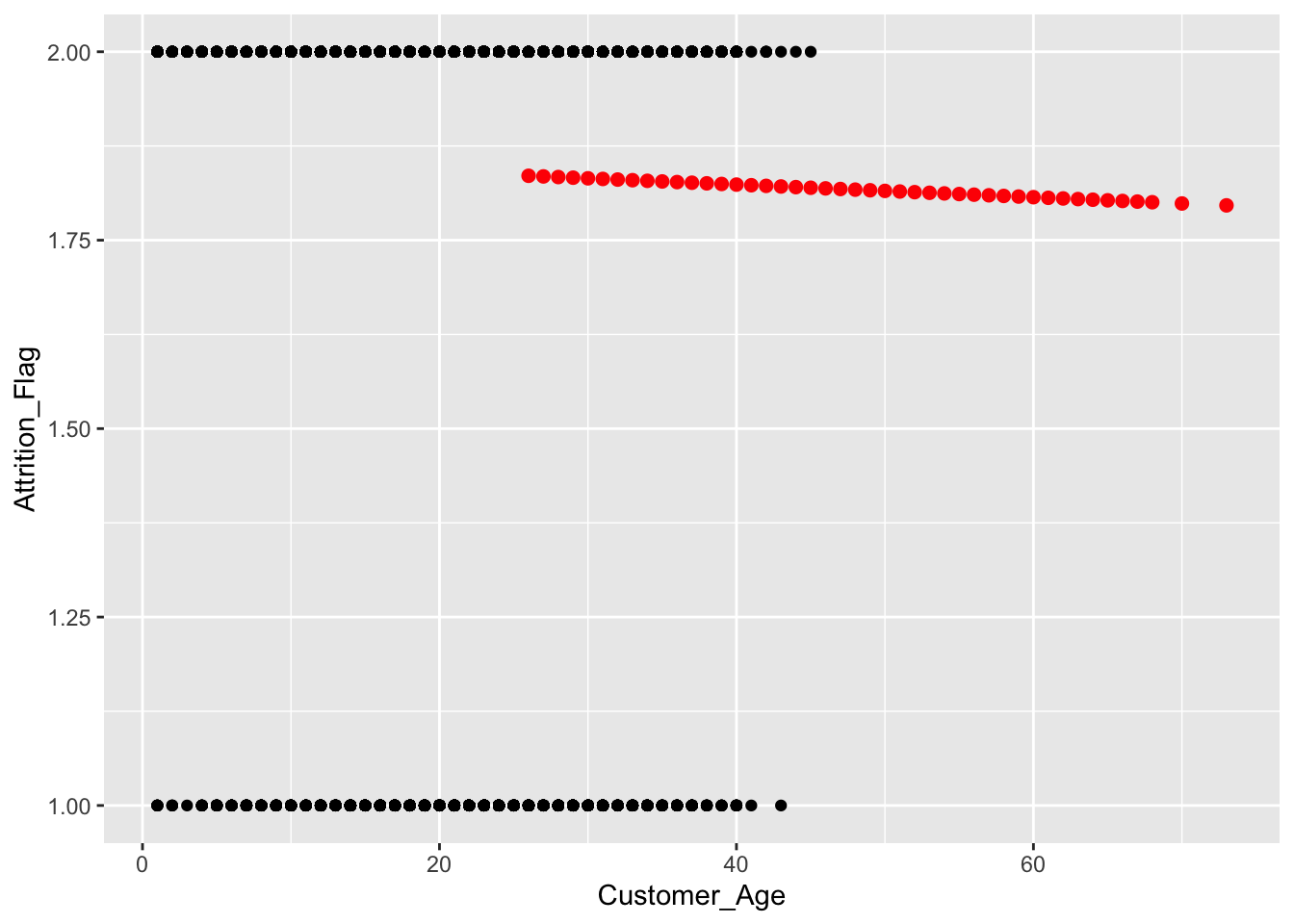
Attrition_Flag[which(Attrition_Flag==2)] <- 0
Bank.lm = glm(Attrition_Flag~Customer_Age+Gender+Education_Level+Marital_Status+Income_Category+Card_Category)
summary(Bank.lm)
##
## Call:
## glm(formula = Attrition_Flag ~ Customer_Age + Gender + Education_Level +
## Marital_Status + Income_Category + Card_Category)
##
## Deviance Residuals:
## Min 1Q Median 3Q Max
## -0.2057 -0.1717 -0.1553 -0.1381 0.8850
##
## Coefficients:
## Estimate Std. Error t value Pr(>|t|)
## (Intercept) 0.1628473 0.0283251 5.749 9.22e-09 ***
## Customer_Age 0.0008081 0.0004553 1.775 0.07595 .
## Gender -0.0282801 0.0086977 -3.251 0.00115 **
## Education_Level 0.0010346 0.0019879 0.520 0.60276
## Marital_Status 0.0093945 0.0049470 1.899 0.05759 .
## Income_Category -0.0007891 0.0028805 -0.274 0.78414
## Card_Category -0.0018264 0.0052833 -0.346 0.72958
## ---
## Signif. codes: 0 '***' 0.001 '**' 0.01 '*' 0.05 '.' 0.1 ' ' 1
##
## (Dispersion parameter for gaussian family taken to be 0.1346583)
##
## Null deviance: 1365.6 on 10126 degrees of freedom
## Residual deviance: 1362.7 on 10120 degrees of freedom
## AIC: 8443.4
##
## Number of Fisher Scoring iterations: 2